Another home advantage blog post.

Motivation

With 92 Premier League games taking place behind closed doors, and considerably more across the globe, there was an abundance of “analysis” claiming that home advantage had completely disappeared or even reversed with games taking place with no fans. I had been looking for a reason to force myself to install and learn Pyro/Numpyro for a while so took this as an opportunity to give it a go.

Model

In a similar fashion to Ben’s analysis here I have used a basic Dixon-Coles style model. The data I used is from a simple XG model, with penalties excluded. I chose to split home advantage into 2 variables;

1. The advantage from playing at your home ground, i.e familiarity with pitch dimensions etc.
2. The advantage gained from atmosphere, i.e fans being present.

Jump to findings

Code

Numpyro code used for the model is below.

def model(team=None, opponent=None, home_id=None, home_fans_id=None, xg=None):
    # Team attack rating.
    attack_mean = numpyro.sample("attack_mean", dist.Normal(0,1))
    attack_sigma = numpyro.sample("attack_sigma", dist.InverseGamma(1,1))
    attack_rating_non_ct = numpyro.sample("attack_rating_non_ct", dist.Normal(0,1).expand([len(set(team))]))
    attack_rate = attack_mean + attack_rating_non_ct[team]*attack_sigma

    # Opponent defense rating.
    defense_mean = numpyro.sample("defense_mean", dist.Normal(0,1))
    defense_sigma = numpyro.sample("defense_sigma", dist.InverseGamma(1,1))
    defense_rating_non_ct = numpyro.sample("defense_rating_non_ct", dist.Normal(0,1).expand([len(set(opponent))]))
    defense_rate = defense_mean + defense_rating_non_ct[opponent]*defense_sigma

    #Advantage from being at home, home_id is 1 whenever team is at home.
    home_attack_basic = numpyro.sample("home_attack_basic", dist.Normal(0,1))
    home_attack_adv = home_id * home_attack_basic

    #Advantage from fans being present, home_fans_id should be 1 when at home and fans are present and 0 when at home with no fans.
    home_attack_fans_basic = numpyro.sample("home_attack_fans_basic", dist.Normal(0,1))
    home_attack_fans = home_fans_id * home_attack_fans_basic

    #Likelihood
    diff = jnp.exp(attack_rate + home_attack_adv + home_attack_fans - defense_rate)
    obs = numpyro.sample("obs", dist.Poisson(diff), obs=xg)

Fitting the model.

nuts_kernel = NUTS(model)
mcmc = MCMC(nuts_kernel, num_warmup=500, num_samples=10000)
rng_key = random.PRNGKey(0)
mcmc.run(rng_key, team=dset.teamid,
         opponent=dset.opponentid,
         home_id=dset.home_id.values,
         home_fans_id=dset.home_fans_present.values,
         xg=dset.xg.values,
         extra_fields=('potential_energy',))

Click here for model summary.

Model summary

parameter	mean	std	median	5.0%	95.0%	n_eff	r_hat
attack_mean	0.15	0.71	0.15	-0.98	1.34	6154.75	1.00
attack_sigma	0.23	0.05	0.23	0.16	0.32	3912.60	1.00
attack_rating_non_ct[0]	1.10	0.52	1.09	0.25	1.95	8374.52	1.00
attack_rating_non_ct[1]	-0.91	0.59	-0.91	-1.90	0.01	11941.38	1.00
attack_rating_non_ct[2]	2.02	0.54	2.01	1.12	2.89	5925.03	1.00
attack_rating_non_ct[3]	-0.14	0.55	-0.13	-1.06	0.75	9457.09	1.00
attack_rating_non_ct[4]	-0.49	0.57	-0.48	-1.44	0.42	12434.17	1.00
attack_rating_non_ct[5]	-0.23	0.56	-0.22	-1.12	0.72	9777.81	1.00
attack_rating_non_ct[6]	-0.18	0.55	-0.18	-1.08	0.72	10686.36	1.00
attack_rating_non_ct[7]	0.14	0.56	0.14	-0.77	1.07	8658.60	1.00
attack_rating_non_ct[8]	0.17	0.54	0.17	-0.68	1.07	10056.12	1.00
attack_rating_non_ct[9]	-1.17	0.60	-1.15	-2.17	-0.23	9568.23	1.00
attack_rating_non_ct[10]	-0.40	0.57	-0.40	-1.29	0.56	11249.37	1.00
attack_rating_non_ct[11]	-0.20	0.55	-0.19	-1.11	0.69	10754.30	1.00
attack_rating_non_ct[12]	-0.28	0.57	-0.27	-1.20	0.68	9816.47	1.00
attack_rating_non_ct[13]	-0.28	0.55	-0.27	-1.21	0.60	10558.21	1.00
attack_rating_non_ct[14]	-0.21	0.55	-0.20	-1.10	0.70	11570.03	1.00
attack_rating_non_ct[15]	-0.79	0.58	-0.77	-1.72	0.19	11271.00	1.00
attack_rating_non_ct[16]	0.17	0.54	0.17	-0.76	1.02	10302.04	1.00
attack_rating_non_ct[17]	0.45	0.54	0.45	-0.48	1.27	9607.86	1.00
attack_rating_non_ct[18]	1.05	0.53	1.04	0.22	1.93	7911.13	1.00
attack_rating_non_ct[19]	0.18	0.54	0.18	-0.70	1.07	9922.93	1.00
defense_mean	-0.13	0.71	-0.14	-1.28	1.04	6149.20	1.00
defense_sigma	0.20	0.05	0.20	0.13	0.28	5284.83	1.00
defense_rating_non_ct[0]	0.71	0.62	0.69	-0.36	1.67	11623.39	1.00
defense_rating_non_ct[1]	-0.84	0.58	-0.83	-1.80	0.09	10142.58	1.00
defense_rating_non_ct[2]	0.99	0.63	0.96	-0.03	2.03	14904.24	1.00
defense_rating_non_ct[3]	-0.76	0.57	-0.75	-1.69	0.19	11255.41	1.00
defense_rating_non_ct[4]	-0.56	0.58	-0.56	-1.51	0.40	10068.25	1.00
defense_rating_non_ct[5]	-0.12	0.59	-0.12	-1.08	0.84	14353.28	1.00
defense_rating_non_ct[6]	0.10	0.60	0.09	-0.84	1.12	11902.51	1.00
defense_rating_non_ct[7]	-0.27	0.58	-0.28	-1.25	0.66	11552.72	1.00
defense_rating_non_ct[8]	0.34	0.61	0.33	-0.66	1.34	14602.78	1.00
defense_rating_non_ct[9]	-0.46	0.57	-0.46	-1.40	0.49	11981.43	1.00
defense_rating_non_ct[10]	-0.16	0.59	-0.17	-1.15	0.79	14187.21	1.00
defense_rating_non_ct[11]	-0.41	0.59	-0.42	-1.37	0.55	10279.23	1.00
defense_rating_non_ct[12]	-1.02	0.57	-1.01	-1.96	-0.11	13133.95	1.00
defense_rating_non_ct[13]	0.09	0.61	0.08	-0.92	1.07	16097.16	1.00
defense_rating_non_ct[14]	-0.10	0.59	-0.10	-1.09	0.86	10490.95	1.00
defense_rating_non_ct[15]	-0.86	0.58	-0.86	-1.81	0.09	11439.39	1.00
defense_rating_non_ct[16]	1.08	0.64	1.07	0.07	2.15	14859.41	1.00
defense_rating_non_ct[17]	0.76	0.63	0.75	-0.22	1.84	11756.59	1.00
defense_rating_non_ct[18]	0.64	0.62	0.63	-0.35	1.68	14086.64	1.00
defense_rating_non_ct[19]	0.92	0.63	0.91	-0.08	1.98	11068.81	1.00
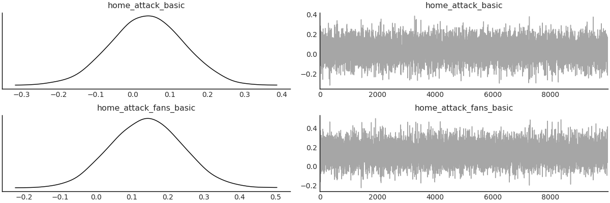
home_attack_basic	0.04	0.10	0.04	-0.12	0.20	8807.34	1.00
home_attack_fans_basic	0.14	0.10	0.14	-0.02	0.30	8699.55	1.00

Parameters

The traceplots for the home advantage parameters are shown below, I will go into more detail about what this means further on.

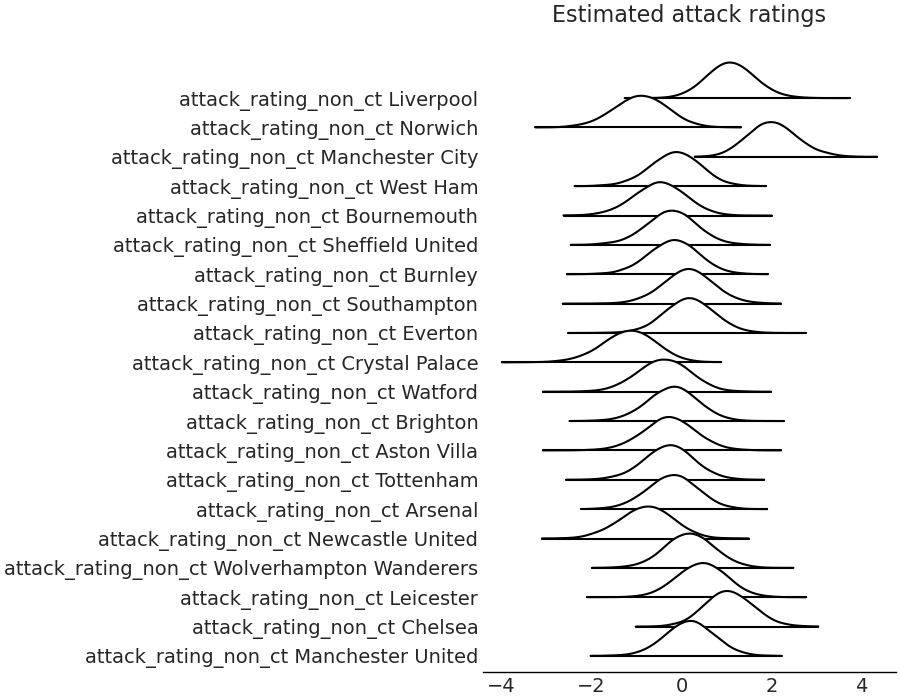
Click here for forest plots of team ratings.

Attack ratings.

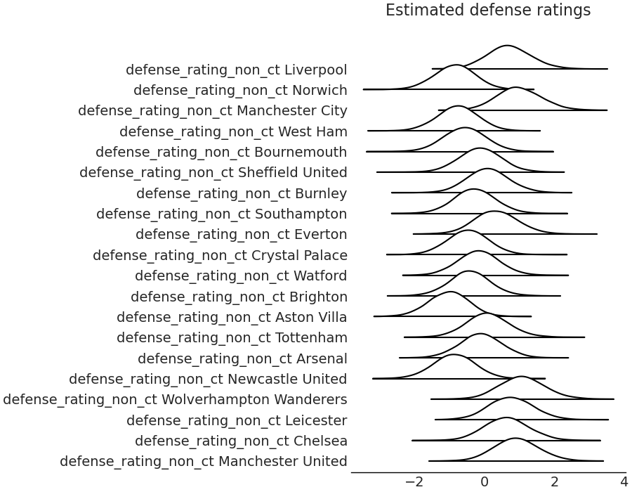
Defense ratings.

Interpretability

We can use the fitted model to look at the difference in predictions between games at home with fans, games at home with no fans, and games at a neutral venue. For example, using the fitted model to predict Manchester City vs Norwich.

Match format	Manchester City goals	Norwich goals
At home with fans	3.0	0.89
At home with no fans	2.62	0.89
Neutral venue	2.51	0.89

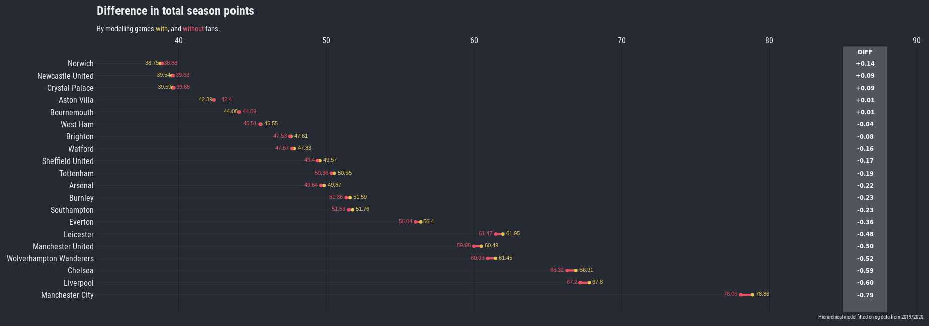
We can then use the fitted model to predict a whole season, and see the difference between a whole season played as normal, and a whole season played behind closed doors.

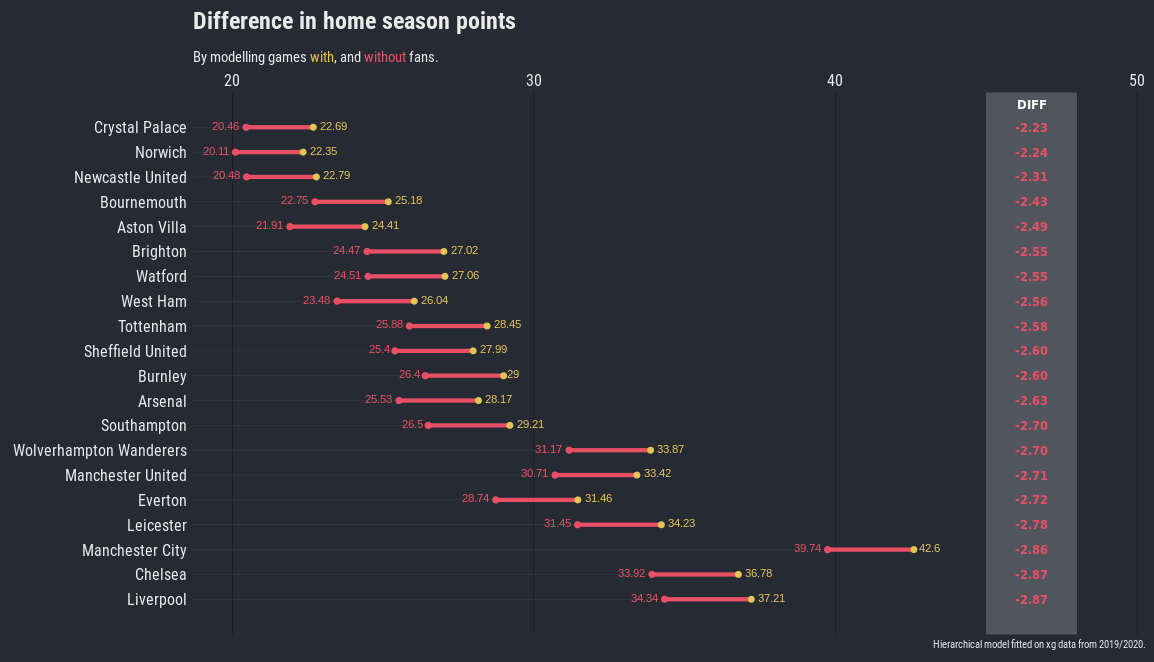
Points

Difference to home season points.

You can see that all teams would earn significantly less points at home over the course of the season if all games were played behind closed doors.

Difference to total season points.

You can see that the majority of teams would earn less points in total over the course of the season, a few of the “worse” teams would earn marginally more points due to the increase in numbers of draws.

Implications

Fans are not due to be allowed back into venues until at least October and even then it is reported to be at only around 30% capacity. If predicting final standings or points for the next season it is important to factor this issue in to get a more accurate prediction.

Model Issues

Looking at the predicted points totals for the top and bottom teams, it is noticeable that the predictions for points seem too low for the good teams and too high for the bad teams. Whilst this was more of an exercise in the impact of no fans at games, this is clearly an issue and I go into details of why the predictions are more conservative than they should be below.

XG model issues.

I have used a basic XG model, which does not include finishing skill, goalkeeper skill, or position of defenders/goalkeeper. This means that good teams will be under-rated and likewise bad teams over-rated. The XG data has penalties excluded, good teams tend to win more penalties than bad teams, again this will under-rate good teams and over-rate bad teams.

Hierarchical model issues.

Hierarchical models inherently suffer from shrinkage. This means that extreme values for teams ratings, i.e the very good, and very bad teams, are pulled towards the grand mean of all the teams.

Other model issues.

The model includes no specific lineup information, squad rotation and January signings are not included as factors. The model assumes that a teams attack & defense abilities are fixed over time, ideally these would be allowed to vary over time however that is a much more difficult coding exercise. There was no accounting for motivational effects, i.e after the restart there was arguably 2 groups of teams, those with high motivation and something to play for (winner/european places/relegation) and those comfortably safe in mid-table.

Future analysis.

Potential continuations listed below.

1. Look at the other European leagues that returned to football behind closed doors and see whether the findings above still hold.
2. Add time varying skill ratings.
3. Include number of fans in the analysis, this will be of interest when fans are allowed back into stadiums at reduced capacity.
4. Include sub groups of good, average and bad teams in the hierarchical model to reduce shrinkage.