

Full code & data for penalty skill post.
Data for the post is available here (player names have been removed).
R & Stan
Load packages
Firstly load the packages necessary for analysis.
library(tidyverse)
library(rstan)
library(bayesplot)
library(RColorBrewer)
Load & inspect data
url <- 'https://raw.githubusercontent.com/markclare1992/markclare1992.github.io/master/assets/pens.csv'
df <- read_csv(url)
#> Parsed with column specification:
#> cols(
#>   match_id = col_character(),
#>   team_id = col_character(),
#>   minute = col_integer(),
#>   second = col_integer(),
#>   taker_id = col_character(),
#>   keeper_id = col_character(),
#>   foot = col_character(),
#>   is_goal = col_logical()
#> )
head(df)
#> # A tibble: 6 x 8
#>   match_id team_id minute second taker_id keeper_id foot  is_goal
#>   <chr>    <chr>    <int>  <int> <chr>    <chr>     <chr> <lgl>
#> 1 x6Qa3Jg  EPkbL       58     37 bEXQP0gd 8zLV8dgY  right TRUE
#> 2 EX1JrQg  Bx4AL       67     26 JEyY1jEk 8zLV8dgY  right TRUE
#> 3 EA328ax  xYnYL       87     21 yx6657x9 8zLV8dgY  right TRUE
#> 4 g9j3yYx  EPkbL       81      8 Ygkjl0Ed 8zLV8dgY  left  TRUE
#> 5 gkMmwkL  Vg9zx       64     58 7EAJkKg4 KZgnMpEp  right FALSE
#> 6 gKpON8x  jL85E       46     33 3EeX1OL4 KZgnMpEp  right TRUE
Grouping by whether or not the penalty is a goal we can look at the average conversion. Here you can see that 75.7% of penalties result in a goal.
df %>%
  group_by(is_goal) %>%
  summarise(n_pens = n()) %>%
  mutate("%" = n_pens/sum(n_pens))
#> # A tibble: 2 x 3
#>   is_goal n_pens   `%`
#>   <lgl>    <int> <dbl>
#> 1 FALSE     2290 0.243
#> 2 TRUE      7134 0.757
Grouping by taker_id we can see the conversion for individual players.
df_player <- df %>%
  group_by(taker_id) %>%
  summarise(n_pens = n(), conversion = mean(is_goal))
df_player %>%
  arrange(-n_pens) %>%
  head(5)
#> # A tibble: 5 x 3
#>   taker_id n_pens conversion
#>   <chr>     <int>      <dbl>
#> 1 Bx47oAg2     87      0.828
#> 2 QEZ1P0Le     58      0.793
#> 3 pEPvQ2xM     55      0.873
#> 4 PLlZq3gM     44      0.75
#> 5 PEjpr2x4     40      0.8
I used ggplot to plot the conversion percentages for players.
ggplot(aes(x=conversion), data=df_player) +
  geom_histogram()
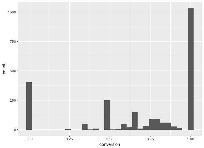
The graph isn’t very clear and doesn’t really show whats happening. You can see that the extreme values of 0% and 100% for conversion percentages have the highest counts.
df_player %>%
  group_by(n_pens) %>%
  summarise(n = n()) %>%
  mutate("%" = n/sum(n)) %>%
  head(5)
#> # A tibble: 6 x 3
#>   n_pens     n    `%`
#>    <int> <int>  <dbl>
#> 1      1  1066 0.419
#> 2      2   446 0.175
#> 3      3   262 0.103
#> 4      4   165 0.0649
#> 5      5   130 0.0511
There is 1066 players in the dataset that have taken only 1 penalty, this is why the conversion graph looks odd.
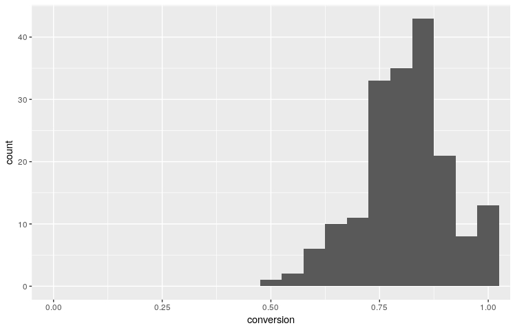
It’s fairly easy to create a graph that provides some insight.
By filtering the dataset for players that have more than 10 attempts, and making the x-axis $$[0,1]$$ a clearer graph is created.
ggplot(aes(x=conversion), data=df_player %>% filter(n_pens>10)) +
  geom_histogram(binwidth = 0.05)+
  coord_cartesian(xlim=c(0,1))
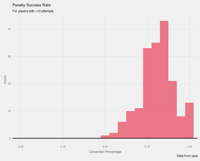
With ggplot2 it’s fairly easy to quickly improve the aesthetics of a graph. I like using a five-thirty-eight style theme from here. Adding titles, axis labels and a horizontal line on the x axis creates the final graph.
ggplot(aes(x=conversion), data=df_player %>% filter(n_pens>10)) +
  geom_histogram(binwidth = 0.05, fill='#E94F64', alpha=.75)+
  coord_cartesian(xlim=c(0,1))+
  fte_theme()+
  geom_hline(yintercept = 0, size=.75)+
  labs(x='Conversion Percentage', y='Count',
       title="Penalty Success Rate",
       subtitle="For players with >10 attempts",
       caption="Data from opta")
Modelling
Complete Pooling
I started off the modelling process using stan in Rstudio (using the rstan package) We have $$N$$ players in the dataset, each player $$n \in N$$ has $$y_{n}$$ goals (successes) out of $$k_{n}$$ penalty attempts (trials). We model each penalty as having the same chance of success $$\phi \in [0,1]$$, hence we assume a uniform prior on $$\phi$$ With the assumption that each players penalty attempts are independent Bernoulli trials and that each player is independent we can use the following stan and R code to fit the distributions.
Stan code (pool.stan)
data {
  int<lower=0> N;           // number players
  int<lower=0> K[N];        // attempts (trials)
  int<lower=0> y[N];        // goals (successes)
}
parameters {
  real<lower=0, upper=1> phi;  // chance of success (pooled)
}
model {
  y ~ binomial(K, phi);
}
R code
library(rstan)
df_binomial <- df %>%
  group_by(taker_id) %>%
  summarise(y = sum(is_goal), K = n())
N <- dim(df_binomial)[1]
K <- df_binomial$K
y <- df_binomial$y
M <- 10000;
fit_pool <- stan("pool.stan", data=c("N", "K", "y"),
                 iter=(M / 2), chains=4);
ss_pool <- rstan::extract(fit_pool);
print(fit_pool, c("phi"), probs=c(0.025, 0.5, 0.975));
Inference for Stan model: pool.
4 chains, each with iter=5000; warmup=2500; thin=1;
post-warmup draws per chain=2500, total post-warmup draws=10000.

    mean se_mean sd 2.5%  50% 97.5% n_eff Rhat
phi 0.76       0  0 0.75 0.76  0.77  3858    1

Samples were drawn using NUTS(diag_e) at Fri Nov 16 12:46:25 2018.
For each parameter, n_eff is a crude measure of effective sample size,
and Rhat is the potential scale reduction factor on split chains (at
convergence, Rhat=1).
You can use the bayesplot package to visualise the parameter estimates.
library(bayesplot)
posterior <- as.matrix(fit_pool)
mcmc_areas(posterior, pars='phi',prob=.975)
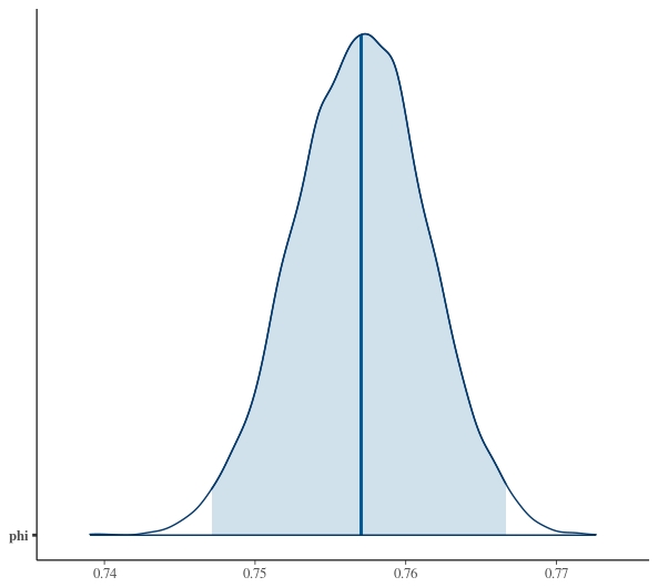
Again it’s fairly easy to customise and improve the look of the graphs more information.
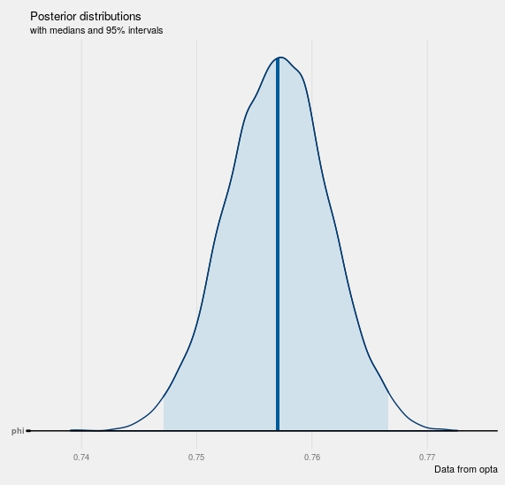
bayesplot_theme_set(fte_theme())
mcmc_areas(posterior, pars='phi',prob=.95) +
  geom_hline(yintercept = 1)+
  labs(title="Posterior distributions",
       subtitle="with medians and 95% intervals",
       caption="Data from opta")
Partial Pooling
Whilst the complete pooling model is a good starting point, it doesn’t seem realistic to assume that each player would have the same probability of scoring a penalty. We assume that each player is part of a population, i.e penalty takers. The properties of the population as a whole are estimated, as are that of the player. Uncertainty based off the different number of attempts for each player will be accounted for. Rather than modelling for chance of success $$\theta_{n} \in [0,1]$$, we model for log-odds $$\alpha_{n}$$. The following logit transform is applied $$\alpha_{n} = {log (\theta_{n}) \over 1 - \theta_{n}}$$. I used a non-centred parameterization as there are lots of players with small counts of penalties taken, using a centred parameterization here would result in a very slow fitting process as the samplers would struggle to explore parameter space. A more in-depth explanation of the maths is available from this extremely useful blogpost, from where I used a lot of ideas.
Stan Code (hier_logit_nc.stan)
data {
  int<lower=0> N;           // number players
  int<lower=0> K[N];        // attempts (trials)
  int<lower=0> y[N];        // goals (successes)
}
parameters {
  real mu;                       // population mean of success log-odds
  real<lower=0> sigma;           // population sd of success log-odds
  vector[N] alpha_std;           // success log-odds
}
model {
  mu ~ normal(1, 1);                             // hyperprior (chosen based on knowledge from complete pooling model)
  sigma ~ normal(0, 1);                           // hyperprior
  alpha_std ~ normal(0, 1);                       // prior
  y ~ binomial_logit(K, mu + sigma * alpha_std);  // likelihood
}
generated quantities {
  vector[N] theta;    // chance of success
  for (n in 1:N)
    theta[n] = inv_logit(mu + sigma * alpha_std[n]);
    //calculate success for non centred parameterization
}
R Code
fit_hier_logit <- stan("hier_logit_nc.stan", data=c("N", "K", "y"),
                       iter=(M / 2), chains=4,
                       control=list(stepsize=0.01, adapt_delta=0.99));
ss_hier_logit <- rstan::extract(fit_hier_logit)
print(fit_hier_logit, c( "mu", "sigma"), probs=c(0.1, 0.5, 0.9));
Inference for Stan model: hier_logit_nc.
4 chains, each with iter=5000; warmup=2500; thin=1;
post-warmup draws per chain=2500, total post-warmup draws=10000.

      mean se_mean   sd  10%  50%  90% n_eff Rhat
mu    1.13       0 0.02 1.10 1.13 1.17 11376    1
sigma 0.18       0 0.09 0.06 0.18 0.29   717    1

Samples were drawn using NUTS(diag_e) at Fri Nov 16 13:25:41 2018.
For each parameter, n_eff is a crude measure of effective sample size,
and Rhat is the potential scale reduction factor on split chains (at
convergence, Rhat=1).
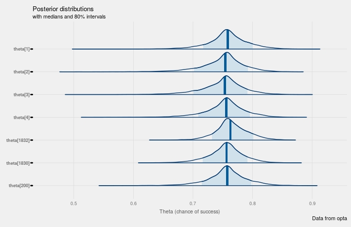
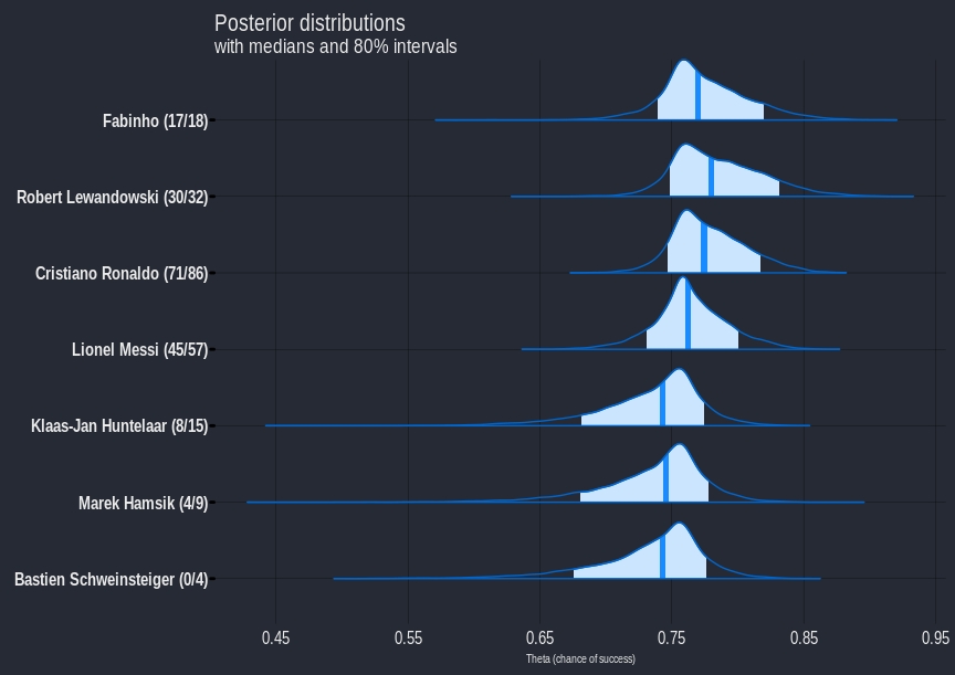
Using bayesplot again we can look at the distributions for players. The fitted parameters can be transformed back into $$\theta_{n}$$, i.e chance of success for players, using the inverse logit transform. I chose a random subset of players as there are a lot of players and it’s impossible to plot them all.
mcmc_areas(posterior_hier, pars=c('theta[1]',
                            'theta[2]',
                            'theta[3]',
                            'theta[4]',
                            'theta[200]',
                            'theta[1830]',
                            'theta[1832]'),
           prob=0.8)+
  labs(x="Theta (chance of success)",
       title="Posterior distributions",
       subtitle="with medians and 80% intervals",
       caption="Data from opta")
Python / PYMC3
I transferred to python to fit the final model. Import the necessary packages.
import numpy as np
import pandas as pd
import matplotlib.pyplot as plt
import theano.tensor as tt
from pymc3 import  Bound, Bernoulli, Model, model_to_graphviz, Normal, sample, sample_ppc, stats, traceplot
import matplotlib.pyplot as plt
Read in the data and convert the taker_id, and keeper_id column to categorical variables. Create arrays of unique takers and keepers from the dataset.
url = 'https://raw.githubusercontent.com/markclare1992/markclare1992.github.io/master/assets/pens.csv'
dat = pd.read_csv(url)
dat['taker_id'] = dat['taker_id'].astype('category')
dat['keeper_id'] = dat['keeper_id'].astype('category')
takers = dat['taker_id'].unique()
keepers = dat['keeper_id'].unique()
We need to convert the taker and player id’s to a nicer format, so that we can map each penalty onto an observation for the taker, the keeper and the outcome.
t_map = {v: k for k, v in enumerate(takers)}
k_map = {v: k for k, v in enumerate(keepers)}
obs_tak = dat['taker_id'].map(t_map).values
obs_keep = dat['keeper_id'].map(k_map).values
obs_wl = dat['is_goal'].values
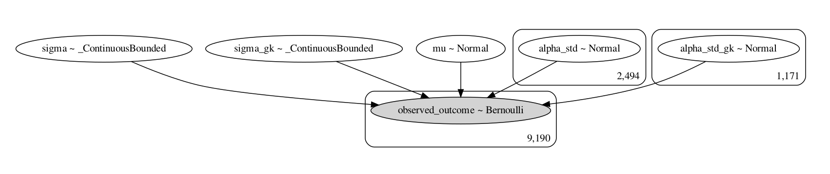
Define the model using pymc3 as follows, the standard deviation parameters (sigma and sigma_gk) have to be restricted to positive only values here because of the subtraction of the taker and keeper skill. I chose to use a different standard deviation parameter for takers and goalkeepers, however a single parameter can be used for both groups and a similar result is found. I used the sigmoid function from the theano library to ensure that $$p \in [0,1]$$.
with Model() as final_model:
    mu = Normal('mu', 1, 1, shape=1)
    BoundedNormal = Bound(Normal, lower=0.0)
    sigma = BoundedNormal('sigma', mu=0, sd=1)
    sigma_gk = BoundedNormal('sigma_gk', mu=0, sd=1)
    alpha_std = Normal('alpha_std', 0, 1, shape=len(takers))
    alpha_std_gk = Normal('alpha_std_gk', 0, 1, shape=len(keepers))
    p = tt.nnet.sigmoid(mu + sigma*alpha_std[obs_tak] - sigma_gk*alpha_std_gk[obs_keep])
    Bernoulli('observed_outcome', p=p, observed=obs_wl)
The model can be visualized by using the graph_to_viz function.
model_to_graphviz(final_model).render('final_model.gv',view=True)
The model can now be fit.
with final_model:
    trace = sample(2000, tune=1000, nuts_kwargs={'target_accept': 0.95})
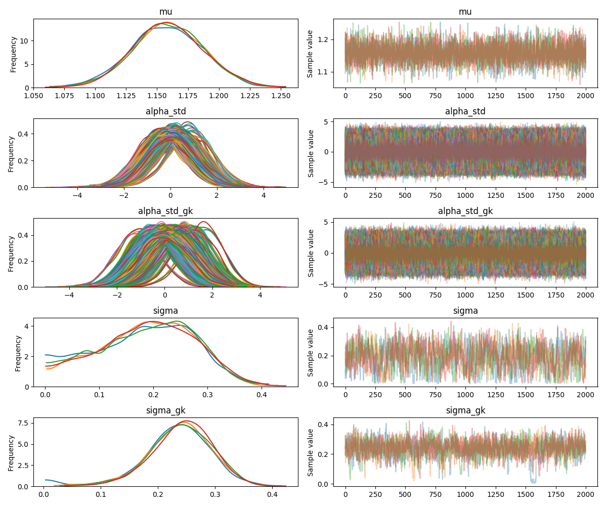
You can see the traceplot by using the code below. The population mean can be recovered from the mu parameter by applying the inverse logit function. This returns a value of approximately 0.76 which fits with the complete pooling model from earlier.
traceplot(trace)
plt.show()
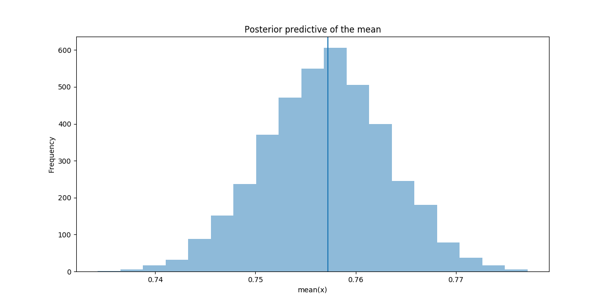
You can sample from the fitted distribution and compare how close the inferred means are to the actual sample mean. This shows how well the model is reproducing patterns found in the real data.
ppc = sample_ppc(trace, samples=4000, model=final_model)
_, ax = plt.subplots(figsize=(12,6))
ax.hist([n.mean() for n in ppc['observed_outcome']], bins=19, alpha=0.5)
ax.axvline(obs_wl.mean())
ax.set(title='Posterior predictive of the mean', xlabel='mean(x)', ylabel='Frequency');
plt.show()
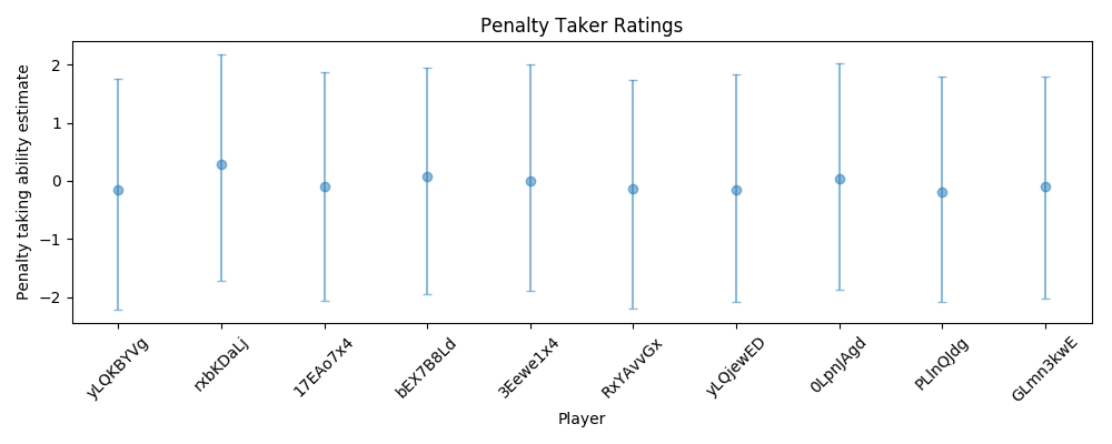
The taker and keeper ratings come from the alpha_std and alpha_std_gk parameters. I used the highest posterior density (hpd) function, (the HPD is the minimum width Bayesian credible interval (BCI)). Again I only plotted a random sample of 10 players as there are too many players. The goalkeeper plot can be created the same way but using the alpha_std_gk parameter instead. The python plots can also be made “prettier” but it’s a bit more time consuming than using ggplot2 from R.
df_hpd = pd.DataFrame(stats.hpd(trace['alpha_std']),
                      columns=['hpd_low', 'hpd_high'],
                      index=takers)

df_median = pd.DataFrame(stats.quantiles(trace['alpha_std'])[50],
                         columns=['hpd_median'],
                         index=takers)

df_hpd = df_hpd.join(df_median)
df_hpd['relative_lower'] = df_hpd.hpd_median - df_hpd.hpd_low
df_hpd['relative_upper'] = df_hpd.hpd_high - df_hpd.hpd_median
df_hpd = df_hpd.sort_values(by='hpd_median')

df_filt = pd.DataFrame.sample(df_hpd, n=10)
df_filt = df_filt.reset_index()
df_filt['x'] = df_filt.index + .5
fig, axs = plt.subplots(figsize=(10,4))
axs.errorbar(df_filt.x, df_filt.hpd_median,
             yerr=(df_filt[['relative_lower', 'relative_upper']].values).T,
             fmt='o', alpha=0.5,capsize=3)

axs.set_title('Penalty Taker Ratings')
axs.set_xlabel('Player')
axs.set_ylabel('Penalty taking ability estimate')
_= axs.set_xticks(df_filt.index + .5)
_= axs.set_xticklabels(df_filt['index'].values, rotation=45)
plt.tight_layout()
plt.show()
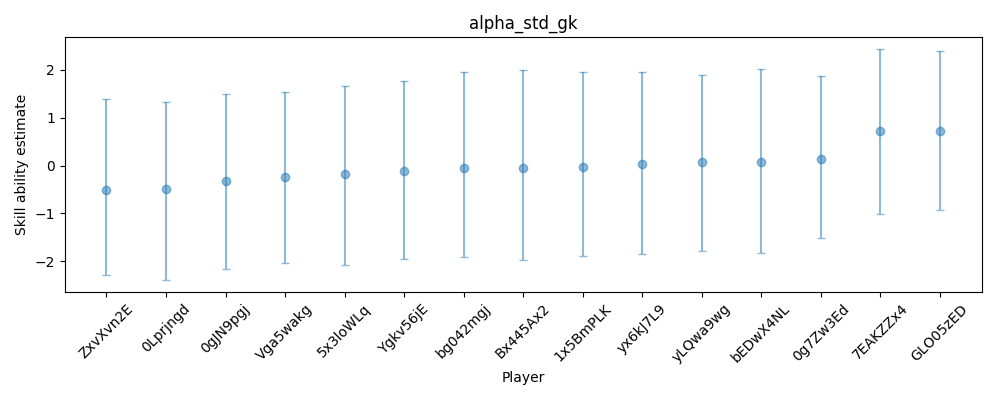
I wrote the plot code as a function to make it easier to generate a new plot.
def plot_trace(trace, parameter, indexes, n_samples):
    """Plot specified parameter from trace"""
    df_hpd = pd.DataFrame(stats.hpd(trace[parameter]),
                          columns=['hpd_low', 'hpd_high'],
                          index=indexes)

    df_median = pd.DataFrame(stats.quantiles(trace[parameter])[50],
                             columns=['hpd_median'],
                             index=indexes)

    df_hpd = df_hpd.join(df_median)
    df_hpd['relative_lower'] = df_hpd.hpd_median - df_hpd.hpd_low
    df_hpd['relative_upper'] = df_hpd.hpd_high - df_hpd.hpd_median
    df_filt = pd.DataFrame.sample(df_hpd, n=n_samples)
    df_filt = df_filt.sort_values(by='hpd_median')
    df_filt = df_filt.reset_index()
    df_filt['x'] = df_filt.index + .5
    fig, axs = plt.subplots(figsize=(10, 4))
    axs.errorbar(df_filt.x, df_filt.hpd_median,
                 yerr=(df_filt[['relative_lower', 'relative_upper']].values).T,
                 fmt='o', alpha=0.5, capsize=3)

    axs.set_title(parameter)
    axs.set_xlabel('Player')
    axs.set_ylabel('Skill ability estimate')
    _ = axs.set_xticks(df_filt.index + .5)
    _ = axs.set_xticklabels(df_filt['index'].values, rotation=45)
    plt.tight_layout()
    plt.show()
plot_trace(trace, alpha_std_gk, keepers, 15)
Leave a Comment